Digital Twin of Human Lungs: Towards Real-Time Simulation and Registration of Soft Organs

Pôle Mécanique - Internal seminar

Alexandre Daby-Seesaram

alexandre.daby-seesaram@polytechnique.edu

LMS, École Polytechnique, Paris, France

Katerina Skardova

katerina.skardova@polytechnique.edu

LMS, École Polytechnique, Paris, France

Martin Genet

martin.genet@polytechnique.edu

LMS, École Polytechnique, Paris, France

March 28, 2025

Idiopathic Pulmonary Fibrosis

The role of mechanics

No identified bio-markers yet
A vicious circle has been hypothesised (F. Liu et al., 2010)
- Fibrotic tissues are stiffer
- Causing higher stresses
- Causing scarring
- Leading to the progress of the disease

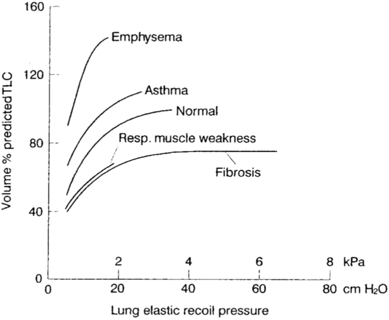
PV curves of healthy and diseased lungs, (Gibson, 2001)

Clinician’s perspective

Rely on mechanical analysis to better understand the disease and its progression

Idiopathic Pulmonary Fibrosis

Inspiration & expiration of diseased lungs

Digital twin from images

Objectives

Improved understanding of the physiological mechanisms

In silico prognostics
- Transfer tools to the clinic
- Patient-specific digital twins

Requirements

Mechanical model of the lung (Patte et al., 2022; Peyraut & Genet, 2024)

Uncertainty quantification (Laville et al., 2023; Peyraut & Genet, (In Revision))

Real-time estimation of the parameters

Lung poro-mechanics (Patte et al., 2022)

Weak formulation :

\[ \begin{cases} \int_{\Omega} \boldsymbol{\Sigma} : d_{\boldsymbol{u}}\boldsymbol{E}\left( \boldsymbol{u^*} \right) ~\mathrm{d}\Omega= W_{\text{ext}}\left(\boldsymbol{u},\boldsymbol{u^*}\right) ~\forall \boldsymbol{u^*} \in H^1_0\left(\Omega \right) \\[4mm] \int_{\Omega} \left(pf + \frac{\partial \Psi \left(\boldsymbol{u},\Phi_f\right)}{\partial \Phi_s}\right) \Phi_f^* ~\mathrm{d}\Omega= 0 ~\forall \Phi_f^* \end{cases} \label{eq:MechPb_lung} \]

Kinematics:

\(\boldsymbol{F} = \boldsymbol{1} + \boldsymbol{\nabla}\boldsymbol{u}\) - deformation gradient
\(\boldsymbol{C} = \boldsymbol{F}^T \cdot \boldsymbol{F}\) - right Cauchy-Green tensor
\(\boldsymbol{E} = \frac{1}{2}\left(\boldsymbol{C} -\boldsymbol{1} \right)\) - Green-Lagrange tensor
- \(I_1 = \text{tr}\left(\boldsymbol{C} \right)\) - first invariant of \(\boldsymbol{C}\)
- \(I_2 = \frac{1}{2} \left(\text{tr}\left(\boldsymbol{C} \right)^2 - \text{tr}\left( \boldsymbol{C}^2 \right) \right)\)

Behaviour

\(\boldsymbol{\Sigma} = \frac{\partial \Psi_s + \Psi_f}{\partial \boldsymbol{E}} = \frac{\partial \Psi_s }{\partial \boldsymbol{E}} + p_f J \boldsymbol{C}^{-1}\) - The second Piola-Kirchhoff stress tensor
- \(p_f = -\frac{\partial \Psi_s}{\partial \Phi_s}\) - fluid pressure
\(\Psi_s\left(\boldsymbol{E}, \Phi_s \right) = W_{\text{skel}} + W_{\text{bulk}}\) \[\begin{cases} W_{\text{skel}} = \beta_1\left(I_1 - \text{tr}\left(I_d\right) -2 \text{ln}\left(\mathrm{det}\left(\boldsymbol{F} \right)\right)\right) + \beta_2 \left(I_2 -3 -4\text{ln}\left(\mathrm{det}\left(\boldsymbol{F} \right)\right)\right) + \alpha \left( e^{\delta\left(\mathrm{det}\left(\boldsymbol{F} \right)^2-1-2\text{ln}\left(\mathrm{det}\left(\boldsymbol{F} \right)\right) \right)} -1\right)\\ W_{\text{bulk}} = \kappa \left( \frac{\Phi_s}{1-\Phi_{f0}} -1 -\text{ln}\left( \frac{\Phi_s}{1-\Phi_{f0}}\right) \right) \end{cases}\]
\(\Phi_s\) current volume fraction of solid pulled back on the reference configurations

Simpler mechanical problem - surrogate modelling

Parametrised (patient-specific) mechanical problem

\[ \definecolor{BleuLMS}{RGB}{1, 66, 106} \definecolor{VioletLMS}{RGB}{77, 22, 84} \definecolor{TealLMS}{RGB}{0, 103, 127} % \definecolor{BleuLMS2}{RGB}{0, 103, 202} \definecolor{BleuLMS2}{RGB}{0, 169, 206} \definecolor{BleuLMPS}{RGB}{105, 144, 255} \definecolor{accentcolor}{RGB}{1, 66, 106} \definecolor{GreenLMS}{RGB}{0,103,127} \definecolor{LGreenLMS}{RGB}{67,176,42} \definecolor{RougeLMS}{RGB}{206,0,55} \]

\[ \boldsymbol{u} = \mathop{\mathrm{arg\,min}}_{H^1\left(\Omega \right)} \int_{\Omega} \Psi\left( \boldsymbol{E}\left(\boldsymbol{u}\left(\textcolor{BleuLMPS}{\boldsymbol{x}}, \textcolor{LGreenLMS}{\left\{\mu_i\right\}_{i \in \mathopen{~[\!\![~}1, \beta \mathclose{~]\!\!]}}}\right)\right) \right) ~\mathrm{d}\Omega- W_{\text{ext}}\left(\textcolor{BleuLMPS}{\boldsymbol{x}}, \textcolor{LGreenLMS}{\left\{\mu_i\right\}_{i \in \mathopen{~[\!\![~}1, \beta \mathclose{~]\!\!]}}}\right) \]

Kinematics:

\(\boldsymbol{F} = \boldsymbol{1} + \boldsymbol{\nabla}\boldsymbol{u}\) - deformation gradient
\(\boldsymbol{C} = \boldsymbol{F}^T \cdot \boldsymbol{F}\) - right Cauchy-Green tensor
\(\boldsymbol{E} = \frac{1}{2}\left(\boldsymbol{C} -\boldsymbol{1} \right)\) - Green-Lagrange tensor
- \(I_1 = \text{tr}\left(\boldsymbol{C} \right)\) - first invariant of \(\boldsymbol{C}\)

Behaviour - Saint Venant-Kirchhoff

\(\Psi = \frac{\lambda}{2} \text{tr}\left(\boldsymbol{E}\right)^2 + \mu \boldsymbol{E}:\boldsymbol{E}\)

Unstable under compression
\(\nu = 0.49\) for quasi-incompressibility
- Soft tissues are often modelled as incompressible materials

Reduced-order model (ROM)

Build a surrogate model
- Parametrised solution \(\left(\textcolor{BleuLMPS}{\boldsymbol{x}}, \textcolor{LGreenLMS}{\left\{\mu_i\right\}_{i \in \mathopen{~[\!\![~}1, \beta \mathclose{~]\!\!]}}}\right)\)
No computations online
On the fly evaluation of the model
- Real-time parameters estimation

Outline

General Surrogate modelling methods and results

Focus on patient-specific shape parametrisation

II - Methods

Mechanical solution interpolation

Reduced-order modelling

Hybrid Neural Network Proper Generalised Decomposition

Preliminary results

Interpolation of the solution

FEM finite admissible space

\[ \mathcal{U}_h = \left\{\boldsymbol{u}_h \; | \; \boldsymbol{u}_h \in \text{Span}\left( \left\{ N_i^{\Omega}\left(\boldsymbol{x} \right)\right\}_{i \in \mathopen{~[\!\![~}1,N\mathclose{~]\!\!]}} \right)^d \text{, } \boldsymbol{u}_h = \boldsymbol{u}_d \text{ on }\partial \Omega_d \right\} \]

Interpretabilty
Kronecker property
- Easy to prescribe Dirichlet boundary conditions

Mesh adaptation not directly embedded in the method

Physics Informed Neural Networks (PINNs)

\[ \boldsymbol{u} \left(x_{0,0,0} \right) = \sum\limits_{i = 0}^C \sum\limits_{j = 0}^{N_i} \sigma \left( \sum\limits_{k = 0}^{M_{i,j}} b_{i,j}+\omega_{i,j,k}~ x_{i,j,k} \right) \]

All interpolation parameters are trainable
Benefits from ML developments

Not easily interpretable
Difficult to prescribe Dirichlet boundary conditions

HiDeNN framework (Y. Liu et al., 2023; Park et al., 2023; Zhang et al., 2021)
- Best of both worlds
- Reproducing FEM interpolation with constrained sparse neural networks
- \(N_i^{\Omega}\) are SNN with constrained weights and biases
- Fully interpretable parameters
- Continuous interpolated field that can be automatically differentiated
- Runs on GPUs

Solving the mechanical problem

Solving the mechanical problems amounts to finding the continuous displacement field minimising the potential energy \[E_p\left(\boldsymbol{u}\right) = \frac{1}{2} \int_{\Omega}\boldsymbol{E} : \mathbb{C} : \boldsymbol{E} ~\mathrm{d}\Omega- \int_{\partial \Omega_N}\boldsymbol{F}\cdot \boldsymbol{u} ~\mathrm{d}A- \int_{\Omega}\boldsymbol{f}\cdot\boldsymbol{u}~\mathrm{d}\Omega. \]

In practice

Compute the loss \(\mathcal{L} := E_p\)
Find the parameters minimising the loss
- Rely on state-of-the-art optimizers (ADAM, LBFGS, etc.)

Degrees of freedom (Dofs)

Nodal values (standard FEM Dofs)
Nodal coordinates (Mesh adaptation)
- hr-adaptivity

r-adaptivity

rh-adaptivity

h-adaptivity: red-green refinement

technical details:

Dofs (initially)	\(569~438\)
Training time (s)	\(7\)
GPU (V100)	1
CPUs	40

Reduced-order modelling (ROM)

Low-rank approximation of the solution to avoid the curse of dimensionality with \(\beta\) parameters

Full-order discretised model

\(N\) spatial shape functions
- Span a finite spatial space of dimension \(N\)
Requires computing \(N\times \beta\) associated parametric functions

Reduced-order model

\(m \ll N\) spatial modes
- Similar to global shape functions
- Span a smaller space
Galerkin projection

Finding the reduced-order basis

Linear Normal Modes (eigenmodes of the structure) (Hansteen & Bell, 1979)
- Do not account for the loading and behaviour specifics
Proper Orthogonal Decomposition (Chatterjee, 2000; Radermacher & Reese, 2013)
- Require wise selection of the snapshots and costly computations
Reduced basis method (Maday & Rønquist, 2002) with EIM (Barrault et al., 2004)
- Rely on prior expensive computations

Proper Generalised Decomposition (PGD)

PGD: (Chinesta et al., 2011; Ladeveze, 1985)

Tensor decomposition

Separation of variables
Low-rank \(m\)
\(\textcolor{BleuLMPS}{\overline{\boldsymbol{u}}_i(\boldsymbol{x})}\) Space modes
\(\textcolor{LGreenLMS}{\lambda_i^j(\mu^j)}\) Parameter modes

\[\textcolor{VioletLMS}{\boldsymbol{u}}\left(\textcolor{BleuLMPS}{\boldsymbol{x}}, \textcolor{LGreenLMS}{\mu}\right) = \sum\limits_{i=0}^{m}\textcolor{BleuLMPS}{\overline{u}_i\left(x\right)}\textcolor{LGreenLMS}{\lambda_i\left(\mu\right)}\]

Discretised problem

From \(N\times N_{\mu}\) unknowns to \(m\times\left(N + N_{\mu}\right)\)
- e.g. \(10000 \times 1000 = 1e7 \gg 5\left( 10 000+ 1000 \right) = 5.5e4\)

Proper Generalised Decomposition (PGD)

PGD: (Chinesta et al., 2011; Ladeveze, 1985)

Tensor decomposition - extra-coordinates

Separation of variables
Low-rank \(m\)
\(\textcolor{BleuLMPS}{\overline{\boldsymbol{u}}_i(\boldsymbol{x})}\) Space modes
\(\textcolor{LGreenLMS}{\lambda_i^j(\mu^j)}\) Parameter modes

\[ \textcolor{VioletLMS}{\boldsymbol{u}}\left(\textcolor{BleuLMPS}{\boldsymbol{x}}, \textcolor{LGreenLMS}{\left\{\mu_i\right\}_{i \in \mathopen{~[\!\![~}1, \beta \mathclose{~]\!\!]}}}\right) = \sum\limits_{i=1}^m \textcolor{BleuLMPS}{\overline{\boldsymbol{u}}_i(\boldsymbol{x})} ~\textcolor{LGreenLMS}{\prod_{j=1}^{\beta}\lambda_i^j(\mu^j)} \]

Discretised problem

From \(N\times\prod\limits_{j=1}^{~\beta} N_{\mu}^j\) unknowns to \(m\times\left(N + \sum\limits_{j=1}^{\beta} N_{\mu}^j\right)\)
- e.g. \(10000 \times 1000^2 = 1e10 \gg 5\left( 10 000+ 2\times 1000 \right) = 6e4\)

Finding the tensor decomposition by minimising the energy \[ \left(\left\{\overline{\boldsymbol{u}}_i \right\}_{i\in \mathopen{~[\!\![~}1,m\mathclose{~]\!\!]}},\left\{\lambda_i^j \right\}_{ \begin{cases} i\in \mathopen{~[\!\![~}1,m\mathclose{~]\!\!]}\\ j\in \mathopen{~[\!\![~}1,\beta \mathclose{~]\!\!]} \end{cases} } \right) = \mathop{\mathrm{arg\,min}}_{ \begin{cases} \left(\overline{\boldsymbol{u}}_1, \left\{\overline{\boldsymbol{u}}_i \right\} \right) & \in \mathcal{U}\times \mathcal{U}_0 \\ \left\{\left\{\lambda_i^j \right\}\right\} & \in \left( \bigtimes_{j=1}^{~\beta} \mathcal{L}_2\left(\mathcal{B}_j\right) \right)^{m-1} \end{cases}} ~\underbrace{\int_{\mathcal{B}}\left[E_p\left(\boldsymbol{u}\left(\boldsymbol{x},\left\{\mu_i\right\}_{i \in \mathopen{~[\!\![~}1, \beta \mathclose{~]\!\!]}}\right), \mathbb{C}, \boldsymbol{F}, \boldsymbol{f} \right) \right]\mathrm{d}\beta}_{\mathcal{L}} \label{eq:min_problem} \]

Proper Generalised Decomposition (PGD)

Building the low-rank tensor decomposition greedily (Ladeveze, 1985; Nouy, 2010)

\[ \boldsymbol{u}\left(\boldsymbol{x}, \left\{\mu_i\right\}_{i \in \mathopen{~[\!\![~}1, \beta \mathclose{~]\!\!]}}\right) = \overline{\boldsymbol{u}}(\boldsymbol{x}) ~\prod_{j=1}^{\beta}\lambda^j(\mu^j) \]

\[ \boldsymbol{u}\left(\boldsymbol{x}, \left\{\mu_i\right\}_{i \in \mathopen{~[\!\![~}1, \beta \mathclose{~]\!\!]}}\right) = \textcolor{RougeLMS}{\sum\limits_{i=1}^{2}} \overline{\boldsymbol{u}}_{\textcolor{RougeLMS}{i}}(\boldsymbol{x}) ~\prod_{j=1}^{\beta}\lambda_{\textcolor{RougeLMS}{i}}^j(\mu^j) \]

\[ \boldsymbol{u}\left(\boldsymbol{x}, \left\{\mu_i\right\}_{i \in \mathopen{~[\!\![~}1, \beta \mathclose{~]\!\!]}}\right) = \sum\limits_{i=1}^{\textcolor{RougeLMS}{m}} \overline{\boldsymbol{u}}_i(\boldsymbol{x}) ~\prod_{j=1}^{\beta}\lambda_i^j(\mu^j) \]

Greedy algorithm

Start with a single mode
Minimise the loss until stagnation

Add a new mode
If loss decreases, continue training

Else stop and return the converged model

The PGD is

An a priori ROM techniques
- Building the model from scratch on the fly
No full-order computations
Reduced-order basis tailored to the specifics of the problem (Daby-Seesaram et al., 2023)

Note

Training of the full tensor decomposition, not only the \(m\)-th mode
Actual minimisation implementation of the PGD
No need to solve a new problem for any new parameter
- The online stage is a simple evaluation of the tensor decomposition

Neural Network PGD

Graphical implementation of Neural Network PGD

\[ \boldsymbol{u}\left(\textcolor{BleuLMPS}{\boldsymbol{x}}, \textcolor{LGreenLMS}{\left\{\mu_i\right\}_{i \in \mathopen{~[\!\![~}1, \beta \mathclose{~]\!\!]}}}\right) = \sum\limits_{i=1}^m \textcolor{BleuLMPS}{\overline{\boldsymbol{u}}_i(\boldsymbol{x})} ~\textcolor{LGreenLMS}{\prod_{j=1}^{\beta}\lambda_i^j(\mu^j)} \]

Interpretable NN-PGD

No black box
- Fully interpretable implementation
- Great transfer learning capabilities
Straightforward implementation
- Benefiting from current ML developments

Straightforward definition of the physical loss using auto-differentiation

def Loss(model,x,detJ,mu):
  
    u = model.space_mode(x)
    eps = torch.autograd.grad(u, x, grad_outputs=torch.ones_like(u))
    lmbda = model.parameter_mode(mu)
    W_int = torch.einsum('ij,ejm,eil,em,mp...,lp...,p->',C,eps,eps,detJ,lmbda,lmbda, mu)

    return 0.5*W_int/mu.shape[0]

Hybridising ROM with NN

Open-source code

pip install NeuROM-Py

All the figures of the papers are in Jupyter’s books
- Greater reproductibility

Stiffness and external forces parametrisation

Illustration of the surrogate model in use (preprint: Daby-Seesaram et al., 2024)

Parameters

Parametrised stiffness \(E\)
Parametrised external force \(\boldsymbol{f} = \begin{bmatrix} ~ \rho g \sin\left( \theta \right) \\ -\rho g \cos\left( \theta \right) \cos\left( \phi \right) \\ \rho g \cos\left( \theta \right) \sin\left( \phi \right) \end{bmatrix}\)

NeuROM

NN-PGD

Immediate evaluation of the surrogate model
Straightforward differentiation capabilities regarding the input parameters

Convergence of the greedy algorithm

Loss convergence

Loss decay

Construction of the ROB

New modes are added when the loss’s decay cancels out
Adding a new mode gives extra latitude to improve predictivity

Accuracy with regards to FEM solutions

Solution	Error
\(E = 3.8 \times 10^{-3}\mathrm{ MPa}, \theta = 241^\circ\)	\(E = 3.8 \times 10^{-3}\mathrm{ MPa}, \theta = 241^\circ\)
\(E = 3.1 \times 10^{-3}\mathrm{ MPa}, \theta = 0^\circ\)	\(E = 3.1 \times 10^{-3}\mathrm{ MPa}, \theta = 0^\circ\)

\(E\) (kPa)	\(\theta\) (rad)	Relative error
3.80	1.57	\(1.12 \times 10^{-3}\)
3.80	4.21	\(8.72 \times 10^{-4}\)
3.14	0	\(1.50 \times 10^{-3}\)
4.09	3.70	\(8.61 \times 10^{-3}\)
4.09	3.13	\(9.32 \times 10^{-3}\)
4.62	0.82	\(2.72 \times 10^{-3}\)
5.01	2.26	\(5.35 \times 10^{-3}\)
6.75	5.45	\(1.23 \times 10^{-3}\)

Multi-level training

Strategy

The interpretability of the NN allows
- Great transfer learning capabilities
  - Start with coarse (cheap) training
  - Followed by fine tuning, refining all modes
Extends the idea put forward by (Giacoma et al., 2015)

Note

The structure of the Tensor decomposition is kept throughout the multi-level training
Last mode of each level is irrelevant by construction
- It is removed before passing onto the next refinement level

Larger Kolmogorov width example

Inhomogeneous stiffness

We parametrise a stiffness jump with a scalar \(\alpha\)
\(E\left(x,y,z\right) = E_1 + \frac{E_2}{2} \left ( 1 + \text{tan}\left( z+\alpha - L \right) \right)\)
The gravity field is still parametrised by two angles \(\theta\) and \(\phi\)
We want to find \[u\left(x, E_1, E_2, \alpha, \theta, \phi \right)\]
with \(100\) sample in each parametric dimension and \(60 000\) spatial dofs
- \(\frac{8\times100^5*60000}{1e9} = 4~800~000\) GB

FENNI-PGD

Sparse encoding of the parametric manifold

Light memory cost
Cheap on the fly evaluation
Access to the fully parametrised solution
- and all its derivative w.r.t. the parameters thanks to autograd

Larger Kolmogorov width example - greedy convergence

Loss convergence

Loss decay

Construction of the ROB

New modes are added when the loss’s decay cancels out
Adding a new mode gives extra latitude to improve predictivity

III - Patient-specific parametrisation

Shape registration pipeline from CT-scans

Building a geometry model from the shapes librairy

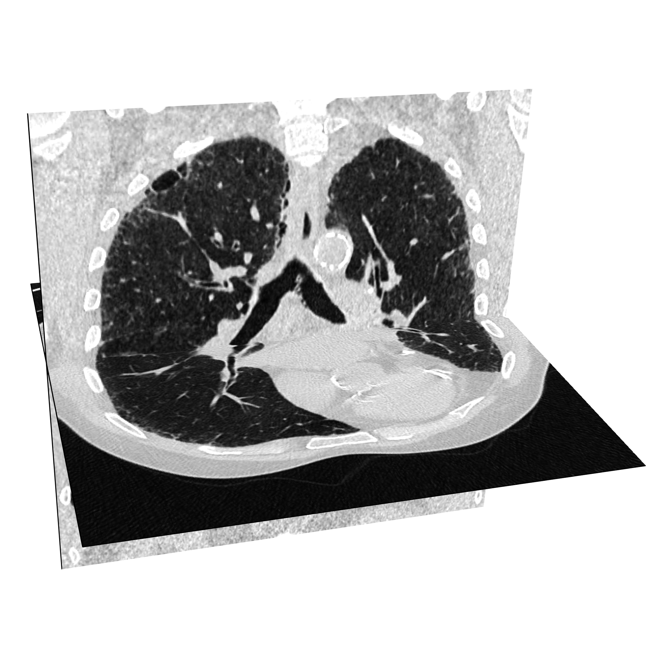
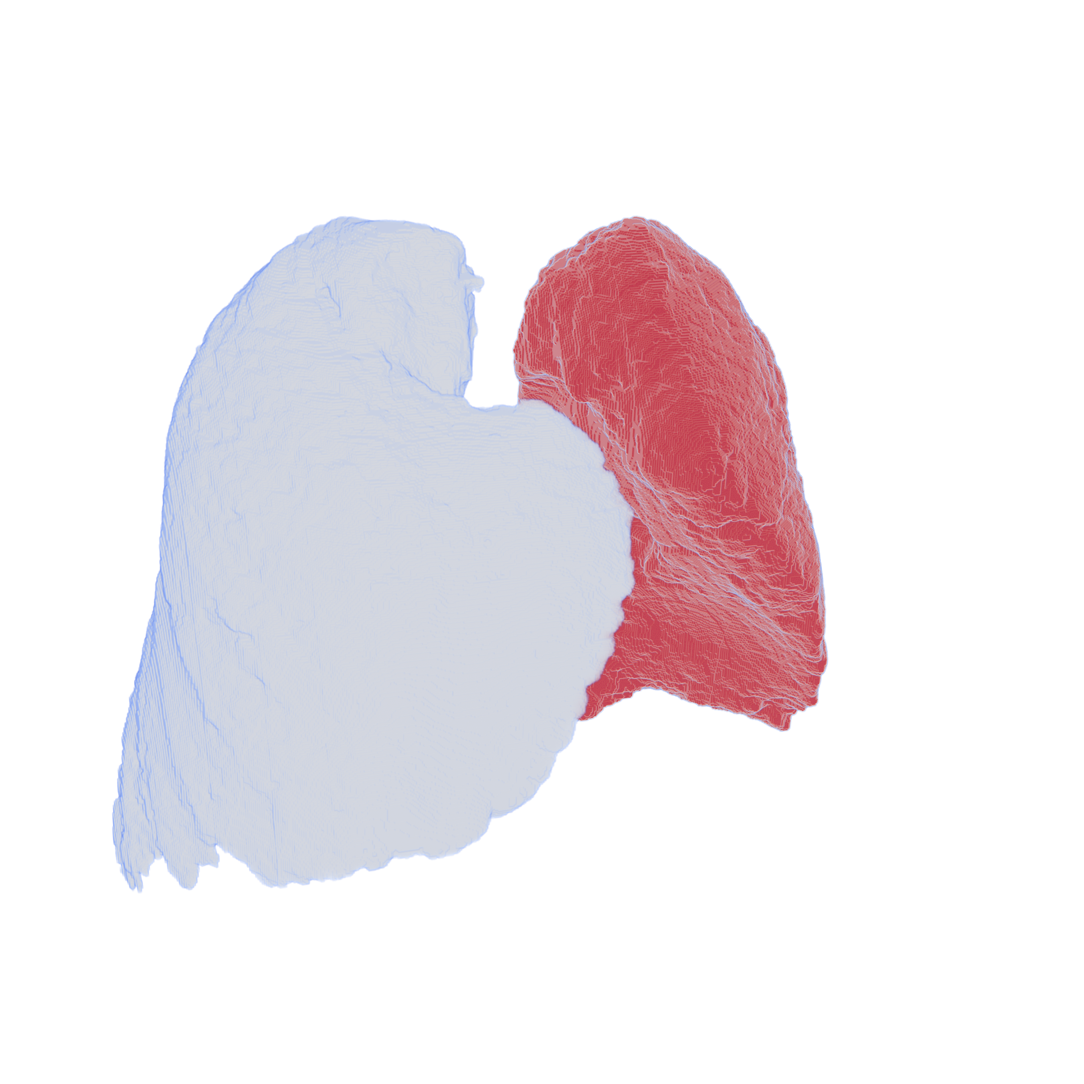
Shape model - available data

CT scans

Raw 3D images

Segmented 3D images

Shape model - registration (Gangl et al., 2021)

Minimisation problem

The objective is to find the domain \(\omega\) occupied by a given segmented shape in a 3D image
Which is solution of

\[\omega = \arg \min\underbrace{ \int_{\omega} I\left( x \right) \mathrm{d}\omega}_{\Psi\left(\omega\right)}\]

With requirement that \(I\left( x \right) \begin{cases} < 0 \forall x \in \mathcal{S} \\ > 0 \forall x \not \in \mathcal{S} \end{cases}\), with \(\mathcal{S}\) the image footprint of the shape to be registered

The domain \(\omega\) can be described by mapping \[\Phi\left(X\right) = I_d + u\left(X\right)\] from a reference shape \(\Omega\), leading to \[\int_{\omega} I\left( x \right) \mathrm{d}\omega = \int_{\Omega} I \circ \Phi \left( X \right) J \mathrm{d}\Omega\]

Shape derivatives

\(D\Psi\left(\omega\right)\left(\boldsymbol{u}^*\right) = \int_{\Omega} \nabla I \cdot u^* J \mathrm{d}\Omega + \underbrace{\int_{\Omega}I \circ \Phi\left(X\right) (F^T)^{-1} : \nabla u^* J \mathrm{d}\Omega}_{\int_{\omega}I\left(x\right) \mathrm{div}\left( u^* \circ \Phi \right) \mathrm{d}\omega}\)
Note that \[\int_{\omega}I\left(x\right) \mathrm{div}\left( u^* \circ \Phi \right) \mathrm{d}\omega = \int_{\partial \omega} I u^* \cdot n \partial \omega\]
- Flat parts of the image result in non-zero derivative of the loss
- The border is “pushed in the right direction”

Sobolev gradient (Neuberger, 1985; Neuberger, 1997)

The regularisation is added through the choice of inner product \(H\) used to reconstruct the gradient

\[D\Psi\left(u\right)\left(v^*\right) = \left(\nabla^H \Psi \left(u\right), v^* \right)_H\]

Classically:
- \(\left(\boldsymbol{u}, \boldsymbol{v}^* \right)_H := \int_{\omega} \boldsymbol{\nabla_s}\boldsymbol{u}:\boldsymbol{\nabla_s}\boldsymbol{\boldsymbol{v}^*}\mathrm{d}\omega + \alpha \int_{\omega} \boldsymbol{u} \cdot \boldsymbol{v^*}\mathrm{d}\omega\)

Shape model - registration (Gangl et al., 2021)

Results

We can

compute mappings from a given shape (a sphere for instance) to the actual patient-specific shape
Get a mapping from a generic lung to patient-specific lungs
- A remove the rigid body motions

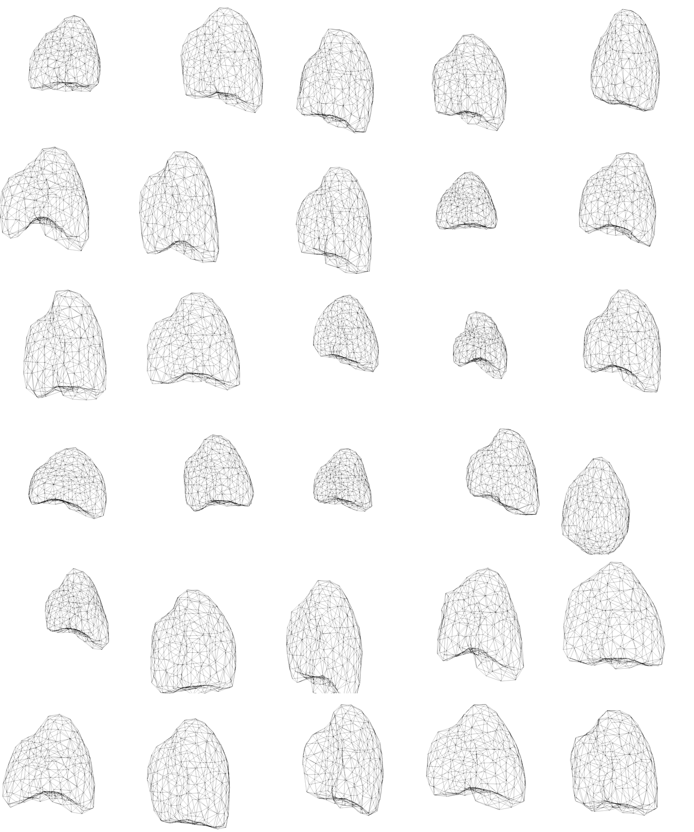
Shape model - parametrisation

Encoding the shape of the lung in low-dimensional spaces

in order to feed the surrogate model we need a parametrisation of the lung
ROM on the shape mappings library

Shape model - parametrisation

Encoding the shape of the lung in low-dimensional spaces

in order to feed the surrogate model we need a parametrisation of the lung
ROM on the shape mappings librairy

Figure 1: lung mappings separability

First investigations - SVD

~40 patients
SVD shows a relatively quick decay of the singular values
Could benefit from non-linear reduction
- k-PCA in perspective
- possibility to use autoencoder

Conclusion

Robust and straightforward general implementation of a NN-PGD
- Interpretable
- Benefits from all recent developments in machine learning
Surrogate modelling of parametrised PDE solution
- Promising results on simple toy case

Perspectives for patient-specific applications

Implementation of the poro-mechanics lung model (Patte et al., 2022)
Further work on parametrising the geometries
Inputting geometry parameters in the NN-PGD
Error quantification on the estimated parameters

Other perspectives

A priori error control of the surrogate model
Sparse/stochastic integration on the parametric hypercube
Enhanced seamless pipeline merging all developments

preprints: (Daby-Seesaram et al., 2024; Škardová et al., 2024)


Github page

References

Barrault, M., Maday, Y., Nguyen, N. C., & Patera, A. T. (2004). An “empirical interpolation” method: Application to efficient reduced-basis discretization of partial differential equations. Comptes Rendus Mathematique, 339(9), 667–672. https://doi.org/10.1016/j.crma.2004.08.006

Chatterjee, A. (2000). An introduction to the proper orthogonal decomposition. Current Science, 78(7), 808–817. https://www.jstor.org/stable/24103957

Chinesta, F., Ladeveze, P., & Cueto, E. (2011). A Short Review on Model Order Reduction Based on Proper Generalized Decomposition. Archives of Computational Methods in Engineering, 18(4), 395–404. https://doi.org/10.1007/s11831-011-9064-7

Daby-Seesaram, A., Fau, A., Charbonnel, P.-É., & Néron, D. (2023). A hybrid frequency-temporal reduced-order method for nonlinear dynamics. Nonlinear Dynamics, 111(15), 13669–13689. https://doi.org/10.1007/s11071-023-08513-8

Daby-Seesaram, A., Škardová, K., & Genet, M. (2024, December 7). Finite Element Neural Network Interpolation. Part II: Hybridisation with the Proper Generalised Decomposition for non-linear surrogate modelling. https://doi.org/10.48550/arXiv.2412.05714

Gangl, P., Sturm, K., Neunteufel, M., & Schöberl, J. (2021). Fully and semi-automated shape differentiation in NGSolve. Structural and Multidisciplinary Optimization, 63(3), 1579–1607. https://doi.org/10.1007/s00158-020-02742-w

Giacoma, A., Dureisseix, D., Gravouil, A., & Rochette, M. (2015). Toward an optimal a priori reduced basis strategy for frictional contact problems with LATIN solver. Computer Methods in Applied Mechanics and Engineering, 283, 1357–1381. https://doi.org/10.1016/j.cma.2014.09.005

Gibson, G. J. (2001). Lung volumes and elasticity. Clinics in Chest Medicine, 22(4), 623–635, vii. https://doi.org/10.1016/s0272-5231(05)70056-3

Hansteen, O. E., & Bell, K. (1979). On the accuracy of mode superposition analysis in structural dynamics. Earthquake Engineering & Structural Dynamics, 7(5), 405–411. https://doi.org/10.1002/eqe.4290070502

Ladeveze, P. (1985). Sur une famille d’algorithmes en mécanique des structures. Sur Une Famille d’algorithmes En Mécanique Des Structures, 300(2), 41–44.

Laville, C., Fetita, C., Gille, T., Brillet, P.-Y., Nunes, H., Bernaudin, J.-F., & Genet, M. (2023). Comparison of optimization parametrizations for regional lung compliance estimation using personalized pulmonary poromechanical modeling. Biomechanics and Modeling in Mechanobiology, 22(5), 1541–1554. https://doi.org/10.1007/s10237-023-01691-9

Liu, F., Mih, J. D., Shea, B. S., Kho, A. T., Sharif, A. S., Tager, A. M., & Tschumperlin, D. J. (2010). Feedback amplification of fibrosis through matrix stiffening and COX-2 suppression. Journal of Cell Biology, 190(4), 693–706. https://doi.org/10.1083/jcb.201004082

Liu, Y., Park, C., Lu, Y., Mojumder, S., Liu, W. K., & Qian, D. (2023). HiDeNN-FEM: A seamless machine learning approach to nonlinear finite element analysis. Computational Mechanics, 72(1), 173–194. https://doi.org/10.1007/s00466-023-02293-z

Maday, Y., & Rønquist, E. M. (2002). A Reduced-Basis Element Method. Journal of Scientific Computing, 17(1), 447–459. https://doi.org/10.1023/A:1015197908587

Neuberger, J. W. (1985). Steepest descent and differential equations. Journal of the Mathematical Society of Japan, 37(2), 187–195. https://doi.org/10.2969/jmsj/03720187

Neuberger, J. W. (1997). Sobolev Gradients and Differential Equations (Vol. 1670). Springer. https://doi.org/10.1007/BFb0092831

Nouy, A. (2010). A priori model reduction through Proper Generalized Decomposition for solving time-dependent partial differential equations. Computer Methods in Applied Mechanics and Engineering, 199(23–24), 1603–1626. https://doi.org/10.1016/j.cma.2010.01.009

Park, C., Lu, Y., Saha, S., Xue, T., Guo, J., Mojumder, S., Apley, D. W., Wagner, G. J., & Liu, W. K. (2023). Convolution hierarchical deep-learning neural network (C-HiDeNN) with graphics processing unit (GPU) acceleration. Computational Mechanics, 72(2), 383–409. https://doi.org/10.1007/s00466-023-02329-4

Patte, C., Genet, M., & Chapelle, D. (2022). A quasi-static poromechanical model of the lungs. Biomechanics and Modeling in Mechanobiology, 21(2), 527–551. https://doi.org/10.1007/s10237-021-01547-0

Peyraut, A., & Genet, M. (2024). Quantification d’incertitudes pour la modélisation pulmonaire per- sonnalisée.

Peyraut, A., & Genet, M. ((In Revision)). Uncertainty quantification for personalized biomechanical modeling: Application to pulmonary poromechanical digital twins. Journal of Biomechanical Engineering.

Radermacher, A., & Reese, S. (2013). A comparison of projection-based model reduction concepts in the context of nonlinear biomechanics. Archive of Applied Mechanics, 83(8), 1193–1213. https://doi.org/10.1007/s00419-013-0742-9

Škardová, K., Daby-Seesaram, A., & Genet, M. (2024, December 7). Finite Element Neural Network Interpolation. Part I: Interpretable and Adaptive Discretization for Solving PDEs. https://doi.org/10.48550/arXiv.2412.05719

Zhang, L., Cheng, L., Li, H., Gao, J., Yu, C., Domel, R., Yang, Y., Tang, S., & Liu, W. K. (2021). Hierarchical deep-learning neural networks: Finite elements and beyond. Computational Mechanics, 67(1), 207–230. https://doi.org/10.1007/s00466-020-01928-9

Appendix - Orthonormalisation of the ROB

To ensure orthonormality of the RON, a Gramm-Schmidt like algorithm can be performed

\[ \boldsymbol{u}_{m+1} = \sum_{i=1}^{m} \underbrace{(\lambda_i + \lambda_{m+1} ~ \overline{\boldsymbol{u}}_i^T \overline{\boldsymbol{u}})}_{\mathring{\lambda}_i} \overline{\boldsymbol{u}}_i + \lambda_{m+1} \underbrace{\left(\overline{\boldsymbol{u}}_{m+1} - \sum_{i=1}^{m} ( \overline{\boldsymbol{u}}_i^T \overline{\boldsymbol{u}}) \overline{\boldsymbol{u}}_i\right)}_{\mathring{\overline{\boldsymbol{u}}}_{m+1}} \]

\[\overline{\boldsymbol{u}}_{m+1} \longleftarrow \frac{\mathring{\overline{\boldsymbol{u}}}_{m+1}}{\Vert\mathring{\overline{\boldsymbol{u}}}_{m+1} \Vert_{\mathbb{K}}} \]

\[ \lambda_{m+1} \longleftarrow \lambda_{m+1} \Vert\mathring{\overline{\boldsymbol{u}}}_{m+1} \Vert_{\mathbb{K}} \] \[ \{\lambda_i\}_{i\in\mathopen{~[\!\![~}1,m\mathclose{~]\!\!]}} \gets \{\mathring{\lambda}_i\}_{i\in\mathopen{~[\!\![~}1,m\mathclose{~]\!\!]}} \]

Much more tricky with more thant 2 parameters in the tensor decomposition

Appendix - PGD of a known field & eigen value problem

Let \(\boldsymbol{u}\left(\boldsymbol{x},t\right)\) defined on \(t \in I = \left[0,T\right]\) and \(\boldsymbol{x} \in \Omega \subset \mathbb{R}^d\). Let’s look at the single mode decomposition: \[\left(\boldsymbol{\overline{u}}_1, \lambda_1\right) = \mathop{\mathrm{arg\,min}}_{\mathcal{U},\mathcal{I}} \left\Vert \boldsymbol{u} - \boldsymbol{\overline{u}}_1 \lambda_1 \right\Vert^2\]

\[\Leftrightarrow\int_{I\times\Omega}\left(\boldsymbol{u} - \boldsymbol{\overline{u}}_1 \lambda_1 \right)\left( \boldsymbol{\overline{u}}^* \lambda^* \right) ~\mathrm{d}\Omega\mathrm{d}t = 0 \forall \lambda^* \in \mathcal{I}, \forall \boldsymbol{\overline{u}}^* \in \mathcal{U}\]

\[\Leftrightarrow\begin{cases} \lambda_1\left(t \right) = \frac{\int_{\Omega}\boldsymbol{u}\left(\boldsymbol{x},t \right)\boldsymbol{\overline{u}}_1 ~\mathrm{d}\Omega}{\int_{\Omega} \boldsymbol{\overline{u}}_1^2 ~\mathrm{d}\Omega} = f\left( \lambda_1 \right) \\ \boldsymbol{\overline{u}}_1\left(\boldsymbol{x} \right) =\frac{\int_{I}\boldsymbol{u}\left(\boldsymbol{x},t \right) \lambda_1 \mathrm{d}t}{\int_{I} \lambda_1^2 \mathrm{d}t} = g\left( \boldsymbol{\overline{u}}_1 \right) \end{cases}\]

\[ \Leftrightarrow \lambda_1 = f \circ g \left( \lambda_1 \right)\]

\[ \Leftrightarrow \underbrace{\int_{\Omega} \boldsymbol{u}\int_{I}\boldsymbol{u}\lambda_1 \mathrm{d}t ~\mathrm{d}\Omega}_{T\left(\lambda_1 \right)} = \underbrace{\frac{\int_{\Omega \left(\int_I \boldsymbol{u}\lambda_1\mathrm{d}t \right)^2 ~\mathrm{d}\Omega}}{\int_I \lambda_1^2\mathrm{d}t}}_ {\omega^2}\lambda_1\]

\(\left\Vert \boldsymbol{u} - \boldsymbol{\overline{u}}_1\lambda_1\right\Vert = \left\Vert \boldsymbol{u}\right\Vert^2 - R\left( \lambda_1 \right)\)

with

\(R\left( \lambda_1 \right) = \omega^2\)

Eigen value problem

Equivalent to searching for the stationarity of a rayleigh’s quotient
It can be shown that minimising the truncation error amounts to fining the largest eigenvalues

In practice

Modes are computed greedily
- Less optimal
The temporal modes can be updated
- improved accuracy

Appendix - Einstein notation

Writing the linear elasticity with the einstein notation:

\[ W_{\text{int}} = \int_{\mathcal{B}}\frac{1}{2} \int_{\Omega}\mathcal{\boldsymbol{\varepsilon}}: \mathbb{C} : \mathcal{\boldsymbol{\varepsilon}}~\mathrm{d}\Omega\mathrm{d}\beta = \frac{1}{2} K_{ij} \mathcal{\boldsymbol{\varepsilon}}_{j}\left(\boldsymbol{\overline{u}}_{em}\right) \mathcal{\boldsymbol{\varepsilon}}_{i}\left(\boldsymbol{\overline{u}}_{el}\right) \mathrm{det}\left(J\right)_{em} \lambda^{\left(1\right)}_{mp} \lambda^{\left(2\right)}_{lp} \lambda^{\left(1\right)}_{mt} \lambda^{\left(2\right)}_{lt} E_p\]

Appendix - Summary of the framework

FENNI-PGD

Appendix - Curse of dimensionality in computing the loss

Computing the non-linear loss using einsum relies on the tensor decomposition and broadcasting to remain efficient
Although the displacement is represented through a tensor decomposition \(\boldsymbol{u}\left(\boldsymbol{x}, \left\{\mu_i\right\}_{i \in \mathopen{~[\!\![~}1, \beta \mathclose{~]\!\!]}}\right) = \boldsymbol{\overline{u}}_i \prod_{j=1}^{\beta}\lambda_i^j(\mu^j)\), some non-linear mapping of that function cannot be easily computed on the independent modes but requires building the full-order solution tensor which leads to prohibitive training costs.

More physically sound behaviour laws

Incompressible Neo-Hookean elastic behaviour: Improve the elastic behaviour \[ \begin{cases} \Psi = C_1(\text{tr}\left(\boldsymbol{C}-\boldsymbol{1}\right)) + f\left(\text{ln}\left(\text{det}\left( \boldsymbol{F}\right) \right) \right)\\[2mm] \left(\text{det}\boldsymbol{F} - 1\right)^2 = 0 \end{cases} \]

Sparse sampling of the hypercube

One idea might be to look at sparse sampling of the parameters sets over which the loss function is computed, using a (greedy) LHS in the parametric space for instance instead of computing the integral of the potential energy over the full parametric hypercube
- Similar idea than in (lu_adaptive_2018?) but applied on PDEs and not data compression
The underlying idea being that the solution interpolation being constrained to be low-rank by the TD, such sparse training might suffice

Heterogeneous stiffness

Bi-stiffness structure with unknown
- Stiffness jump \(\Delta E\)
- Jump position \(\alpha\)

Towards the parametrisation of the disease’s progression
- Can be adapted to different stages of the diseases
- Different physiological initial stiffness

Heterogeneous stiffness

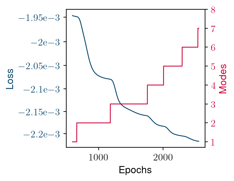
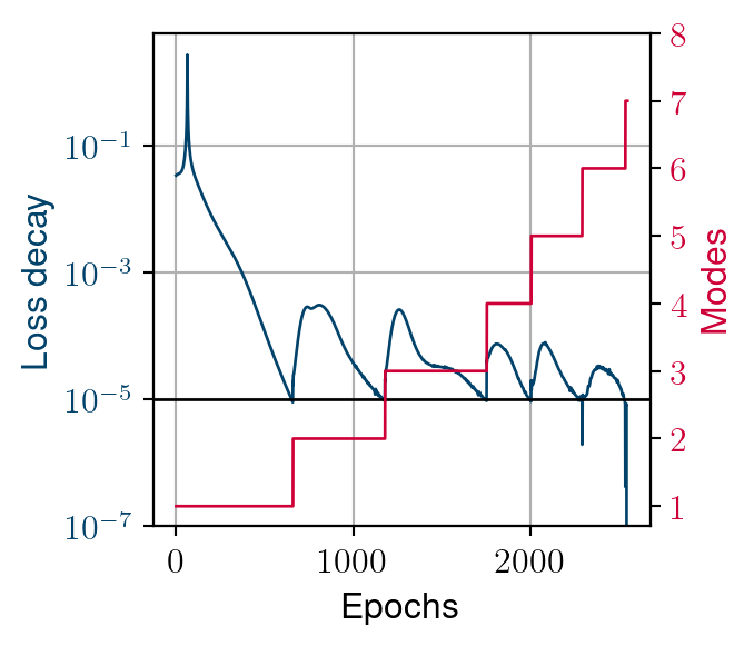
Convergence process

Larger Kolmogorov n-with’s example
Similar behaviour in constructing the reduced-order basis
- Adding a mode leads to a recovery in loss decay
- This recovery decreases until global stagnation